3D graphics in Resolver One using OpenGL and Tao, part II: an orrery

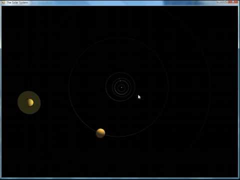
In my last post about animated 3D graphics in Resolver One (the souped-up spreadsheet the company I work for makes), I showed a bouncing, spinning cube controlled by the numbers in a worksheet. Here's something more sophisticated: a 3D model of the planets in our solar system, also know as an orrery (click the image for video):

:

To try this one out yourself:

• If you didn't already do so for part I, download and install the Tao Framework, a set of multimedia libraries that (among many other things) makes it easy for .NET programs like Resolver One to call the OpenGL 3D graphics libraries.
• Again, if you don't have it already, download Resolver One. (It's free to try.)
• Get the sample spreadsheet, along with its supporting Python code. Unzip this file somewhere, and then open the file orbits.rsl with Resolver One.

A window showing the 3D animation of the solar system will appear when the file loads. To manipulate it, drag the mouse left/right to spin the solar system around the Y axis, or up/down to spin around the X axis (left to right in the initial state). Zoom in and out using the mouse wheel or +/-.

Here's how it works in more detail; I'll start with the spreadsheet and then go on to the OpenGL/Tao/IronPython support code that lives in OpenGLPlanets.py later.

The Planets worksheet

The Planets sheet of the spreadsheet is mostly static data, which (as I said in the video) is largely copied from Wikipedia. I shan't waste time here explaining exactly what an orbit's semimajor axis, inclination to the Sun's equator, longitude of the ascending node or argument of perihelion are because you can easily look them up -- or, even better, you can read this excellent tutorial on How to Calculate the Positions of the Planets, which I found halfway through building the spreadsheet and wish I'd found before I started.

The "Rings function" column in the Planets sheet uses the fact that Resolver One can store any kind of data in a cell to store one function per planet. Not the results of the function, but a pointer to the function itself, so that it can be passed around and called elsewhere by code that needs it. Just to make things a little bit more difficult for those who aren't comfortable with functional programming, the way I've implemented this is by writing a function that takes the parameters of the rings (internal and external radii and angle to the planet's orbit) and then returns a function that will draw rings with those parameters. So we have a cell that calls a function that returns a function that is then stored in that cell. All clear? Good.

(The only planet that has a rings function is, of course, Saturn. You might want to experiment with adding rings to other planets -- I think most of the gas giants have rings of some sort. In fact, perhaps a better name for this would be "Decorator function", because the function that is specified here can draw anything at all -- an interesting variation might be to modify it to draw the Earth's Moon. I'll leave that as an exercise for the reader...)

Moving briskly on to the other columns in the "Planets" sheet, we have the number of days in each "tick". When plotting an orbit, we divide it into a given number of points (700 is the default); a "tick" is the amount of time it takes the planet to get from one tick to the next. (The first version of this orrery plotted a point for every (Earth) day, so there were 88 ticks in Mercury's orbit, 224 or so in Venus', 365-odd for Earth, and... well, things got a little hairy when it came to Pluto's 248-year orbit.) Anyhow, this number is used when calculating the orbits. An interesting side-point -- instead of being calculated by formulae, it's calculated by a loop in the pre-formulae user code. This is to handle a rather complex dependency issue that I shan't explain here, though if anyone's interested I can give details in the comments.

After the "days/tick" column, we just have a few columns whose sole purpose is to convert the user-friendly degrees in which we have entered some of the orbital parameters into math-function-friendly radians. These are done in the same pre-formulae code as the "days/tick" calculations, for the same dependency-related reason.

The other worksheets

Now let's move on to the worksheets for the planets. They're all basically the same, so let's look at the one for Mercury as an example. Working through the columns one by one:

• A holds one value, in cell A1. This is a reference to the row that represents the planet in the Planets sheet, and is populated by user code which we'll look at later.
• B holds an ascending sequence starting with 0, one number for every point in the planet's orbit -- in other words, one for each tick in time for which we need to calculate a point. Apart from its header, it's also populated from user code.
• C contains a sequence of times, starting with zero. These are the times around the orbit for which we will be calculating points later on, and are calculated with a column-level formula (click on the row header to see it) that combines data from the row that is stored in A1 (and thus ultimately references the Planets sheet) and the values in the ticks column, B. It looks like this: =float(#tick#_) * A1["days/tick"]
• D through J are a series of column-level formulae, each building on the previous ones and bringing in other values from A1. They basically work through the calculations that you will see on the page I recommended earlier: How to Calculate the Positions of the Planets. The details of each calculation is delegated to one of a set of Python functions that are defined in the pre-formula user code, and the final results are those in rows H-J -- a series of x, y and z locations that describe the planet's motion.

And that's it for the worksheets. Now, on to the user code.

The pre-constants user code

Look at the blue section in the code editor that is below the spreadsheet grid for this code. It starts off with a definition of the number of points we want to calculate per orbit. The default of 700 means that it takes 14 seconds to calculate everything for every planet on my (not very speedy) machine; you can increase this to get smoother animations with slower calculation times, and decrease it if you don't mind the planets leaping their way around their orbits.

The code then goes on to define the functions that do the heavy lifting for the column-level formulae that we looked at earlier in the per-planet worksheets. calculateMeanAnomaly, calculateTrueAnomaly, calculateOrbitalDistance, calculateX, calculateY, and calculateZ are all simple enough (and did I mention that there's a great web page describing how they work?), but calculateEccentricAnomaly is a little complicated. The problem is that we have a value called the mean anomaly (M), another called the eccentricity (ε), and we want to work out the eccentric anomaly (E), but the equation that relates them is:

M = E - εsin(E)

If you can't see how to rearrange that so that it tells you how to get E, given a value for M, you're not alone. The equation is transcendental, and there is no simple solution. Instead, we have to use a numerical method to work out a best-guess value for E. calculateEccentricAnomaly uses the Newton–Raphson method to do this, generating a result of E that is correct to within 5 decimal places.

The pre-constants code finishes off with the function used for rings; it takes the angle to the planet's orbit, and inner and outer radii for the rings, and returns a function that draws the rings. This function in turn takes a parameter that tells it how much to scale the radii -- this value is calculated by the main OpenGL code in OpenGLPlanets.py, which we'll come to later.

The pre-formulae user code

Further down the code editor window you will find this user code section, with a green background. It calculates various values that the formulae in the spreadsheet will use.

It consists of a loop through the worksheets defining individual planets; for each, it:

• Finds the associated row in the Planets worksheet.
• Puts a reference to that row into the planet's own worksheet.
• Fills in the four columns in the Planets worksheet that I mentioned earlier needed to be calculated by user code: "days/tick" and the various "such-and-such in radians" columns.
• Puts pointsPerOrbit rows into the planet's worksheet's "tick" column.

Once this is all done, there is enough information for the column-level formulae in the planets' worksheets to calculate the detailed orbits.

The post-formulae user code

This is very similar in structure to the code in my last post; we import the OpenGL code used to display the planets, check if we already have an open graphics window, and create one if we don't.

Next, we clear the window's list of planets to draw, and then iterate over the worksheets that contain planet data. For each one we create a new Planet object populated with the calculated positions for the orbit and with the other details of the planet -- radius, colour, ring function, and so on -- and add that to the window's list of planets. Once that's done, the window can display the orbits.

That's everything in the spreadsheet. Now, let's look at the supporting OpenGL code in OpenGLPlanets.py.

The IronPython support code

I won't go into this is huge amounts of detail; there are many good OpenGL tutorials and references out there, and duplicating stuff that's already been done much better would be a waste! In addition, much of what's in there is the same as the code in my last post, and was explained there. So, a quick run through the new bits in the code:

• After importing the libraries we'll need, we set up a few constants defining the colour of the sunlight and the location of the Sun in our orrery (bright yellow and in the middle respectively).
• We define some properties for the reflective properties of the planets.
• We cache a specific overload of the glLightfv function. This is a workaround for what appears to be a memory leak in IronPython; in the original version of the code, I was calling this overloaded version of the function directly inside the method that draws the orrery — that is, once per frame. The simulation would start off fine, but within a few tens of minutes would run out of memory and crash. After much investigation I discovered that the cause was this overloaded function, and that caching the overload fixed the problem.
• Next, we define a Planet class, which we created instances of from within the spreadsheet's post-formulae code. This class has several useful features:
  • It keeps all of the properties relating to each planet together.
  • It lets us package up the knowledge of how to draw the planet when we are a specific number of days into the simulation, in a method sensibly called draw. A little more detail about how we do that: let's say we're 1,000 days into the simulation and we want to draw Venus. At 700 ticks/orbit, Venus has roughly 0.32 days/tick, so 1,000 days in, we are on the 1,000/0.32 = 3,125th tick. The planet's positions list contains one orbit's worth of points, one per tick, so we need the 3,125th item in that list. Of course, there are only 700 points in the list, but because each orbit leads into another identical one, we can take 3125 modulo 700 to work out the index, and get the 325th item in the list. This gives us the x, y and z coordinates we need, and then it's just a case of making the appropriate OpenGL calls to draw a sphere of the right colour in the right place, and calling the rings function if there is one.
  • In addition, the draw function generates a number of points, one for each position in the positions list. This is how the tracks of the orbits are displayed, in the orrery — a helpful guide for the eye so that a viewer can easily see where each planet is going.
• Once the Planet class has been defined, we have the OrreryWindow. This is actually very similar to the SpinningBoxWindow I described in my last post. The main differences:
  • __init__ adds event handlers that are used to track mouse drags and button presses so that you can rotate and zoom the display; most of that (including the event handlers themselves futher down) should be pretty self-explanatory. (Post a comment with any questions if it's not!)
  • __init__ also moves a few of the parameters passed in to OpenGL's Glu.gluPerspective function (specifically, near, far, fovY, and fovYU) into class fields, purely for the sake of clarity. Play with these if you want to see the image re-constituted with, say, a fish-eye lens (by increasing fovY) or a zoom lens (by decreasing it).
  • Finally, __init__ sets up and later code tracks how many days we are into the simulation, and how many days we should advance for each repaint of the orrery.
  • After __init__ we have the new mouse and key event handlers, and then come createDrawingContext, killGLWindow, resizeGLScene, and Show, which are completely unchanged except for the move to using fields instead of embedded constants for the call to Glu.gluPerspective in resizeGLScene.
  • Next, initGL, which no longer needs to load textures, but does now create a light to represent the Sun. It's not all that different from the previous one, though.
  • Next come goToSun and cameraDistance, which are basically just helper functions for draw.
  • draw is significantly simpler than its counterpart in my previous post, as all it needs to do is draw the Sun (there's a bit of cleverish code in there to make sure that the Sun's radius expands to make sure it's visible even from so far away that OpenGL would normally not show it) and then iterate through the planets and tell each one to draw itself.
  • And we finish off the OrreryWindow class with its run method, which is completely unchanged from the one in the previous example.
• Finally, at the bottom of OpenGLPlanets.py, we have CreateBackgroundOrreryWindow, which creates an OrreryWindow and sets it up with its own .NET event loop. This is pretty much unchanged from the previous example, though I've added some slightly better exception handling — .NET produces pretty alarming error messages if an unhandled exception is thrown by a background thread, so it's good to always catch and display them before that happens.

And that's it! Hopefully that was all clear, but if anything needs more explanation, please do leave a comment and I'll clarify things as much as I can.